4.10 Application: The Game of Life

The game of Life, devised by British mathematician John H. Conway, is a Solitaire-type game that is analogous with "the rise, fall and alternations of a society of living organisms." The game, which is actually a zero-player game, was first introduced by Martin Gardner in his Mathematical Games column in the October 1970 issue of Scientific American. Since its introduction, Life has attracted much attention and has been widely studied as it can be used to observe how complex systems or patterns can evolve from a simple set of rules. The game of Life was an early example of a problem in the modern field of mathematics called cellular automata.

Rules of the Game

The game uses an infinite-sized rectangular grid of cells in which each cell is either empty or occupied by an organism. The occupied cells are said to be alive, whereas the empty ones are dead. The game is played over a specific period of time with each turn creating a new "generation" based on the arrangement of live organisms in the current configuration. The status of a cell in the next generation is determined by applying the following four basic rules to each cell in the current configuration:

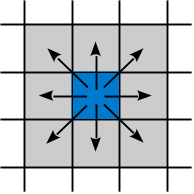
1. If a cell is alive and has either two or three live neighbors, the cell remains alive in the next generation. The neighbors are the eight cells immediately surrounding a cell: vertically, horizontally, and diagonally.
   
2. A living cell that has no live neighbors or a single live neighbor dies from isolation in the next generation.
3. A living cell that has four or more live neighbors dies from overpopulation in the next generation.
4. A dead cell with exactly three live neighbors results in a birth and becomes alive in the next generation. All other dead cells remain dead in the next generation.

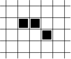
The game starts with an initial configuration supplied by the user. Successive generations are created by applying the set of rules simultaneously to each cell in the grid. Interesting patterns can develop as the population of organisms undergoes changes by expanding or eventually dying out. To illustrate the game of Life, consider the following simple configuration of live organisms:

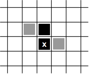
Applying the rules to this configuration creates the next generation. This results in two organisms dying (shown below as the light gray boxes) based on rule 2, one remaining alive based on rule 1, and the generation of a new organism based on rule 4 (the black box marked with an x).

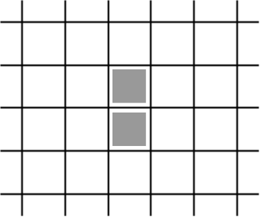
If we evolve the next generation, the system dies out since both live cells in the first generation have a single live neighbor.

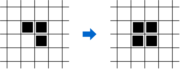
While some systems may eventually die out, others can evolve into a "stable" state. Consider the following initial configuration and its first generation. The result is a stable state since the four live cells each have three neighbors and no dead cell has exactly three neighbors in order to produce a new live cell.

Another interesting patterns is the "two-phase oscillator," which alternates between successive generations:

Designing a Solution

The game of Life requires the use of a grid for storing the organisms. A Life Grid ADT can be defined to add a layer of abstraction between the algorithm for "playing" the game and the underlying structure used to store and manipulate the data.

We now develop a program for the game of Life using the Life Grid ADT. The implementation of the program provided below was developed using a top-down design consisting of several functions. The main routine creates the game grid and evolves new generations of organisms. It relies on two additional functions: draw and evolve.

The draw routine, the implementation of which is left as an exercise, prints a text-based representation of the game grid. The evolve function generates a new configuration of organisms based on the rules of the game. A list is used within evolve to store the coordinates of live cells in the next generation. After iterating over all the cells, the grid is reconfigured using this list of coordinates. This is necessary since the current configuration stored in the game grid cannot be modified with the next generation until the neighbor count has been computed for each cell in the current generation.

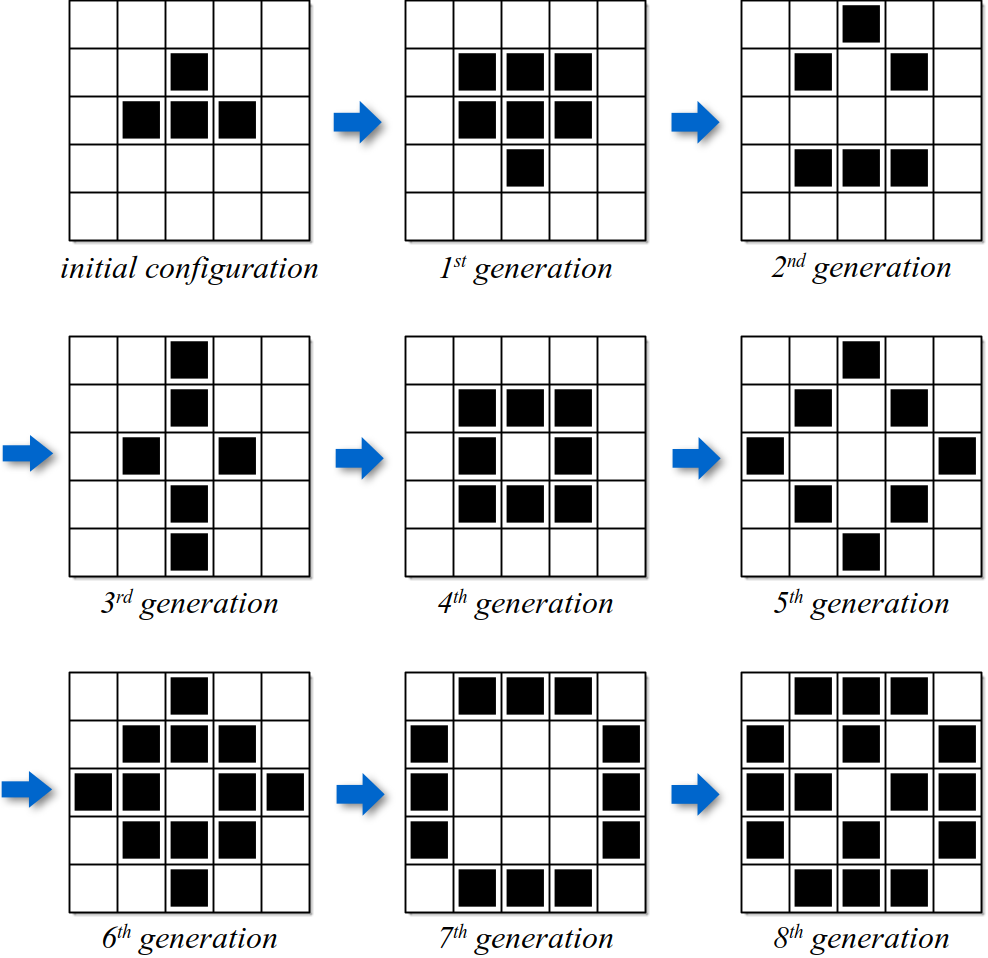
The program also defines several constant variables. These are used to specify the grid size, the number of generations to be created, and the set of initial live cells. Using constant variables allows for easy modifications to any of these parameters as needed without having to modify other parts of the program. Of course, this information could be extracted from the user or a text file instead. The results of executing the gameoflife program are illustrated graphically in Figure 4.10.1.

Figure 4.10.1: The results of using the gameoflife program on a sample grid configuration. Configurations after the eighth generation produce a two-phase oscillator, alternating between the configuration of the seventh and eighth generations.

Implementation

The actual game of Life specifies a rectangular grid of infinite size. When developing a computer solution for such a problem, we are limited to grids of a fixed size. The game of Life can still be implemented, however, by using a finite size for the grid. If the system grows too large where it does not fit into the space, it can be "played" again, with a larger grid.

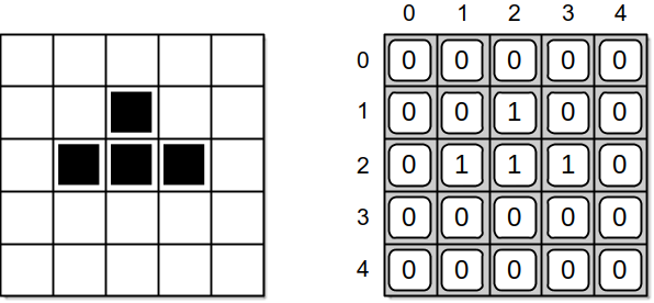
Before implementing the LifeGrid class, we must decide how the data should be organized and select an appropriate structure. The most obvious is the use of a two-dimensional array to represent the grid. Next, we must decide what values to store in the grid to represent the organisms, both dead and alive. Any pair of values can be used. We are going to use the value 0 to represent the dead cells and the value 1 for the live cells. This choice is based on the ease it creates when counting the number of neighbors for a given cell. Figure 4.10.2 illustrates the abstract and physical views of the game grid.

Figure 4.10.2: The game grid representation with live and dead cells: (left) the abstract view and (right) the physical view using a 2-D array of 0's and 1's.

The implementation of the LifeGrid class is provided below. At the top of the class definition, before specifying the constructor, two constant variables are initialized to store the values used to mark the cells within the game grid. These constants are defined within the class itself and outside of the methods since they are not actual data fields of a LifeGrid object. By using the named constants, the code is easier~to read and the values used to represent the cell status could easily be changed if we were so inclined.

NOTE
	Constant variables defined within a class are actually class variables that are unique to the class and not to individual objects. To reference a class constant variable, you use the name of the class in place of the self keyword. For example, the command print(GameGrid.DEAD_CELL) would be used to print the value of the DEAD_CELL class variable.

The constructor, shown in lines 10-14, creates a 2-D array for the grid using the Array2D class defined earlier in the chapter. The cells are cleared as the ADT definition requires by calling the configure method with an empty coordinate list. The grid dimension accessor methods are easily implemented using the corresponding methods of the Array2D class. The three cell modification routines are also straightforward. Note that the ADT definition requires the cell indices specified for the clearCell and setCell methods must be valid. Since this is also the precondition required of the Array2D element access methods, we omit the direct specification of assertions in these methods. The configure method, shown in lines 25-29, clears the grid cells by setting each to a dead organism. It then iterates through the coordinate list and uses the setCell method to set the live cells.

The numLiveNeighbors method is left as an exercise. Note, however, since we used the integer values 0 and 1 to represent the state of a cell, counting the number of live neighbors is as simple as summing the contents of the neighboring cells. Working with a fixed-size grid introduces the problem of how to deal with the cells around the border. A border cell will not have all eight neighbors since some of them lie outside the grid. Different approaches can be taken when a border cell is examined. The most common is to assume any neighboring cell lying outside the grid contains a dead organism.