5.5 Amortized Cost

The append operation of the list structure introduces a special case in algorithm analysis. The time required depends on the available capacity of the underlying array used to implement the list. If there are available slots, a value can be appended to the list in constant time. If the array has to be expanded to make room for the new value, however, the append operation takes linear time. When the array is expanded, extra capacity is added that can be used to add more items without having to immediately expand the array. Thus, the number of times the append operation actually requires linear time in a sequence of $n$ operations depends on the strategy used to expand the underlying array.

Consider the problem in which a sequence of $n$ append operations are performed on an initially empty list, where $n$ is a power of $2$.

Suppose the array is doubled in capacity each time it has to be expanded and assume the size of the underlying array for an empty list has the capacity for a single item. We can tally or compute the total running time for this problem by considering the time required for each individual append operation. This approach is known as the aggregate method since it computes the total from the individual operations.

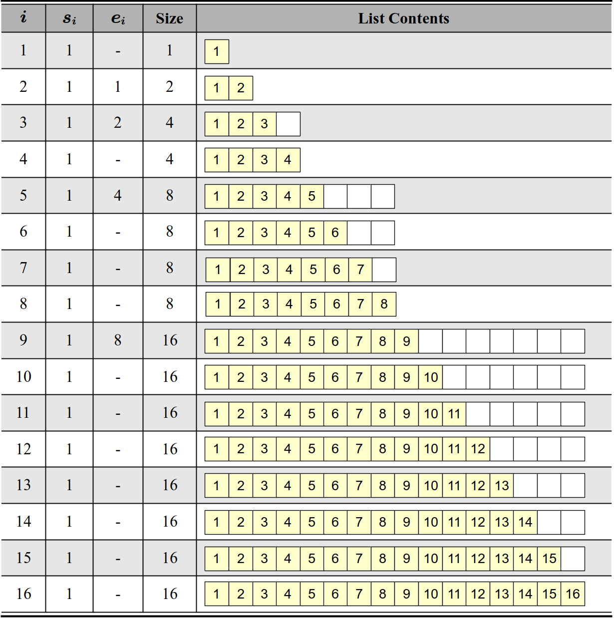
Figure 5.5.1 illustrates the aggregate method when applied to a sequence of $16$ append operations. $s_i$ represents the time required to physically store the $i^{\text{th}}$ value when there is an available slot in the array or immediately after the array has been expanded. Storing an item into an array element is a constant time operation. $e_i$ represents the time required to expand the array when it does not contain available capacity to store the item. Based on our assumptions related to the size of the array, an expansion only occurs when $i-1$ is a power of $2$ and the time incurred is based on the current size of the array ($i-1$). While every append operation entails a storage cost, relatively few require an expansion cost. Note that as the size of $n$ increases, the distance between append operations requiring an expansion also increases.

Figure 5.5.1: Using the aggregate method to compute the total run time for a sequence of

Based on the tabulated results in Figure 5.5.1, the total time required to perform a sequence of $16$ append operations on an initially empty list is $31$, or just under $2n$. This results from a total storage cost ($s_i$) of $16$ and a total expansion cost ($e_i$) of $15$. It can be shown that for any $n$, the sum of the storage and expansion costs, $s_i+e_i$, will never be more than $T(n)=2n$. Since there are relatively few expansion operations, the expansion cost can be distributed across the sequence of operations, resulting in an amortized cost of $T(n)=2n⁄n$ or $\text{O}\left(1\right)$ for the append operation.

WARNING

Amortized Cost Is Not Average Case Time Do not confuse amortized cost with that of average case time. In average case analysis, the evaluation is done by computing an average over all possible inputs and sometimes requires the use of statistics. Amortized analysis computes an average cost over a sequence of operations in which many of those operations are "cheap" and relatively few are "expensive" in terms of contributing to the overall time.

Amortized analysis is the process of computing the time-complexity for a sequence of operations by computing the average cost over the entire sequence. For this technique to be applied, the cost per operation must be known and it must vary in which many of the operations in the sequence contribute little cost and only a few operations contribute a high cost to the overall time. This is exactly the case with the append method. In a long sequence of append operations, only a few instances require $\text{O}\left(n\right)$, while many of them are $\text{O}\left(1\right)$. The amortized cost can only be used for a long sequence of append operations. If an algorithm used a single append operation, the cost for that one operation is still $\text{O}\left(n\right)$ in the worst case since we do not know if that's the instance that causes the underlying array to be expanded.